Algorithm Complexity Growth with Big-O Notation
Not so long ago, I was asked by one of the developers what the big deal is with “big-O notation.” The source of confusion for this relatively straightforward concept was all the definitions and mathematical vocabulary around it. While I do agree that we should be strict and demand correctness, there are certain areas and terms that can be relaxed a bit and explained in simpler language. Let’s see what Wikipedia says:
Big O notation is a mathematical notation that describes the limiting behavior of a function when the argument tends towards a particular value or infinity.
It’s true, I agree. It is correct, but too complex. Some people may find it hard to wrap their heads around it. We can rephrase it to be more accessible, but still correct:
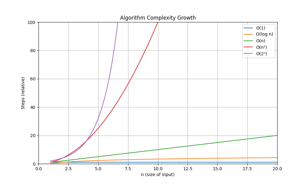
Big O notation is a way to describe how efficient an algorithm is. When we calculate the Big O, the final result tells us how the number of steps or operations grows as the input size increases. Don’t mix algorithm complexity with execution time - Big O will not give us that information.
Let’s take a look at some typical examples:
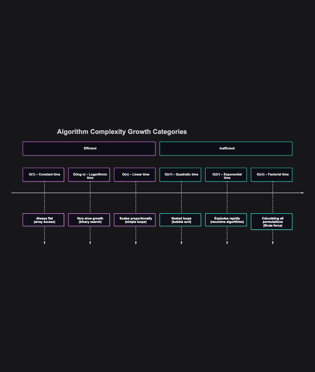
Example 1: O(1) - Constant Time
function GetElementAtIndex(arr: array of Integer; i: Integer): Integer;
begin
  Result := arr[i];
end;
In this example, no matter how big the array is, we always perform the same number of operations (just one), to get the element at a given index. Therefore, this function has a time complexity of O(1), which means it runs in constant time. Constant time means it will always take the same number of steps to complete, regardless of the input size.
Example 2: O(n) - Linear Time
function FindMaximum(arr: array of Integer): Integer;
var
  i: Integer;
  maxValue: Integer;
begin
  if Length(arr) = 0 then
    raise Exception.Create('Array is empty.');

  maxValue := arr[0];

  for i := 1 to High(arr) do
    if arr[i] > maxValue then
      maxValue := arr[i];

  Result := maxValue;
end;
If the size of the array (n) increases, the number of operations we perform also increases linearly. Linear time means that if we double the size of the input, the time it takes roughly doubles as well.
Example 3: O(n²) - Quadratic Time
procedure BubbleSort(var arr: array of Integer);
var
  i, j, n, temp: Integer;
begin
  n := Length(arr);
  for i := 0 to n - 1 do
    for j := 0 to n - i - 2 do
      if arr[j] > arr[j + 1] then
      begin
        temp := arr[j];
        arr[j] := arr[j + 1];
        arr[j + 1] := temp;
      end;
end;
As the size of the array increases, the number of operations grows quadratically. Quadratic time means that if we double the size of the input, the time taken increases by a factor of four (2²). It has steep growth even for small input sizes.
Example 4: O(log n) - Logarithmic Time
function BinarySearch(arr: array of Integer; target: Integer): Integer;
var
  left, right, mid: Integer;
begin
  left := 0; right := High(arr);
  while left <= right do
  begin
    mid := (left + right) div 2;
    if arr[mid] = target then
    begin
      Result := mid;
      Exit;
    end;
    if arr[mid] < target then
      left := mid + 1
    else
      right := mid - 1;
  end;
  Result := -1;
end;
Logarithmic time is very efficient for large datasets because, even as the input size grows, the number of operations increases very slowly. Each time we double the size of the input, we only add one additional operation.
Example 5: O(2ⁿ) - Exponential Time
function Fibonacci(n: Integer): Integer;
begin
  if n <= 1 then
    Result := n
  else
    Result := Fibonacci(n - 1) + Fibonacci(n - 2);
end;
Exponential time “explodes” very quickly as the input size increases. Even for small values of n, the number of operations becomes enormous.
| n | O(1) | O(log n) | O(n) | O(n²) | O(2ⁿ) |
|---|---|---|---|---|---|
| 10 | 1 | ~3 | 10 | 100 | 1024 |
| 100 | 1 | ~7 | 100 | 10,000 | ~10³⁰ |
| 1000 | 1 | ~10 | 1000 | 1,000,000 | ~10³⁰¹ |
What’s the big deal with Big O Notation?
Well, apparently if we know the complexity of our algorithms, and it hurts performance, or even costs us money, we can try to optimize it. How do we know that something is better? By comparing the complexities. The correct path forward is to either change the algorithm or to reorganize the data structures we use. This is not only some fancy math, it has practical applications.
For example, we can use Big O to decide which indexing strategy is better to use in the OpenSearch. We are not going to jump into that rabbit hole now, but we are going to look into the basic indexing and how it relates to Big O notation.
Data Structures and Algorithm Complexity
Once upon a time, phonebooks were large printed books that contained names and addresses. Depending on the area they covered, they could be quite large. We will take a small step into the past… sort of.
Look at the list of UNSORTED phonebook name entries below and try to find “Huey Duck”:
Jerry Jr.
SpongeBob RoundPants
Gadget Hackwrench
Garry Oak
Bart Simpson
Jerome Mouse
Dale
Gale Oak
Homer Simpleton
Pinky 2
Ed
SpongeBob SquarePants
Tommy Cat
Edd
The Brain
Daisy Duck
Yakko Warner
Thomas O'Malley
Donald Duck
Dot Warner
Wakko Warner
SpongeBob NoPants
Bratt Simpson
Gary Oak
Pinky
Homer Simian
Dewey Duck
Ash Ketchum
Tom Cat
Eddy
Huey Duck
Jerry Mouse
Homer Simpson
Darkwing Duck
Monterey Jack
Chip
Launchpad McQuack
Louie Duck
Not easy, right? We have to go through each name entry one by one until we find the one we’re looking for. Searching in a table without a suitable index is O(n) because the database has to scan all rows.
Is there a way to improve this? Of course there is, and some of you are probably already screaming the solution: “Sort that list!” Yes, we can sort the phonebook entries alphabetically.
Ash Ketchum
Bart Simpson
Bratt Simpson
Chip
Dale
Daisy Duck
Darkwing Duck
Dewey Duck
Donald Duck
Dot Warner
Ed
Edd
Eddy
Gale Oak
Gadget Hackwrench
Garry Oak
Gary Oak
Homer Simian
Homer Simpleton
Homer Simpson
Huey Duck
Jerry Jr.
Jerry Mouse
Jerome Mouse
Launchpad McQuack
Louie Duck
Monterey Jack
Pinky
Pinky 2
SpongeBob NoPants
SpongeBob RoundPants
SpongeBob SquarePants
The Brain
Thomas O'Malley
Tom Cat
Tommy Cat
Wakko Warner
Yakko Warner
If we have the same task as before, but the data is now sorted alphabetically, what will our approach be?
In this example, to find “Huey Duck”:
- Jump to “Homer Simpleton” in the middle of the list. Since “Huey Duck” comes after “Homer Simpleton” alphabetically, we can ignore the top half of the list.
Homer Simpson
Huey Duck
Jerry Jr.
Jerry Mouse
Jerome Mouse
Launchpad McQuack
Louie Duck
Monterey Jack
Pinky
Pinky 2
SpongeBob NoPants
SpongeBob RoundPants
SpongeBob SquarePants
The Brain
Thomas O'Malley
Tom Cat
Tommy Cat
Wakko Warner
Yakko Warner
We repeat this process until we find the name we are looking for.
- Jump to the middle of the bottom half, which is “Pinky 2.” Since “Huey Duck” comes before “Pinky 2” alphabetically, we can ignore the bottom half.
Homer Simpson
Huey Duck
Jerry Jr.
Jerry Mouse
Jerome Mouse
Launchpad McQuack
Louie Duck
Monterey Jack
Pinky
- We jump to the middle of that section, which is “Jerome Mouse.” Since “Huey Duck” comes before “Jerome Mouse” alphabetically, we can ignore the bottom half.
Homer Simpson
Huey Duck
Jerry Jr.
Jerry Mouse
- We jump to the middle of that section, which is “Huey Duck.”
No more splits, we found it!
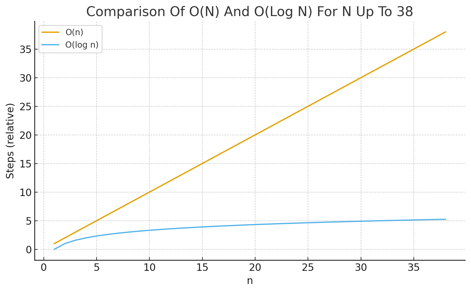
Congratulations, you have just performed a binary search, and it has O(log n) complexity. Much better than O(n), right? Not convinced? Let’s compare the two approaches in the table below:
| Complexity | Given n = 38 | Meaning |
|---|---|---|
| O(n) | 38 | Scanning all 38 items (worst case) |
| O(log n) | ≈ 5.25 | ceil(5.25) = 6 steps using binary search |
Searching unindexed data is not efficient. For small datasets, this may not be an issue, but as the dataset grows in size, it can become serious performance and resource consuming bottleneck. To ilustrate this, let’s look into the example of 1,000,000 entries:
| Complexity | n = 1,000,000 | Meaning |
|---|---|---|
| O(n) | 1,000,000 | Scanning all 1,000,000 items (worst case) |
| O(log n) | ≈ 19.93 | ceil(19.93) = 20 steps using binary search |
As we can see, the difference between the two is humongous. We need only 20 steps on indexed data, compared to 1,000,000 document reads! If this is not a good reason to learn more advanced techniques for applying Big-O, then I don’t know what is.
Conclusion
We touched on many different areas and concepts while explaining Big-O, which is a good thing. It shows how each piece of math, algorithms, and technology fits together when architecting solutions, designing database indexes, or writing efficient code. Understanding Big-O isn’t very useful unless we also know how, and where, to apply it.